1. Dijkstra
Dijkstra's algorithm is an algorithm for finding the shortest paths between nodes in a graph, which may represent, for example, road networks. It was conceived by computer scientist Edsger W. Dijkstra in 1956 and published three years later.
The algorithm exists in many variants; Dijkstra's original variant found the shortest path between two nodes, but a more common variant fixes a single node as the "source" node and finds shortest paths from the source to all other nodes in the graph, producing a shortest-path tree.
Suppose you would like to find the shortest path between two intersections on a city map: a starting point and a destination. Dijkstra's algorithm initially marks the distance (from the starting point) to every other intersection on the map with infinity. This is done not to imply there is an infinite distance, but to note that those intersections have not yet been visited; some variants of this method simply leave the intersections' distances unlabeled. Now, at each iteration, select the current intersection. For the first iteration, the current intersection will be the starting point, and the distance to it (the intersection's label) will be zero. For subsequent iterations (after the first), the current intersection will be the closest unvisited intersection to the starting point (this will be easy to find).
From the current intersection, update the distance to every unvisited intersection that is directly connected to it. This is done by determining the sum of the distance between an unvisited intersection and the value of the current intersection, and relabeling the unvisited intersection with this value (the sum), if it is less than its current value. In effect, the intersection is relabeled if the path to it through the current intersection is shorter than the previously known paths. To facilitate shortest path identification, in pencil, mark the road with an arrow pointing to the relabeled intersection if you label/relabel it, and erase all others pointing to it. After you have updated the distances to each neighboring intersection, mark the current intersection as visited, and select the unvisited intersection with lowest distance (from the starting point) - or the lowest label-as the current intersection. Nodes marked as visited are labeled with the shortest path from the starting point to it and will not be revisited or returned to.
Continue this process of updating the neighboring intersections with the shortest distances, then marking the current intersection as visited and moving onto the closest unvisited intersection until you have marked the destination as visited. Once you have marked the destination as visited (as is the case with any visited intersection) you have determined the shortest path to it, from the starting point, and can trace your way back, following the arrows in reverse; in the algorithm's implementations, this is usually done (after the algorithm has reached the destination node) by following the nodes' parents from the destination node up to the starting node; that's why we keep also track of each node's parent.
This algorithm makes no attempt to direct "exploration" towards the destination as one might expect. Rather, the sole consideration in determining the next "current" intersection is its distance from the starting point. This algorithm therefore expands outward from the starting point, interactively considering every node that is closer in terms of shortest path distance until it reaches the destination. When understood in this way, it is clear how the algorithm necessarily finds the shortest path. However, it may also reveal one of the algorithm's weaknesses: its relative slowness in some topologies.
Testing with sample input map
map = false(10);
% Add an obstacle
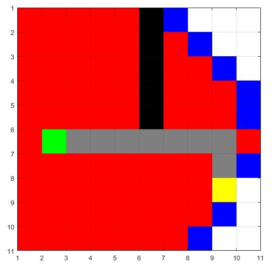
map (1:5, 6) = true;
start_coords = [6, 2];
dest_coords = [8, 9];
%%
close all;
[route, numExpanded] = DijkstraGrid (map, start_coords, dest_coords);
 ---->
---->
function [route,numExpanded] = DijkstraGrid (input_map, start_coords, dest_coords)
% Run Dijkstra's algorithm on a grid.
% Inputs :
%   input_map : a logical array where the freespace cells are false or 0 and
%   the obstacles are true or 1
%   start_coords and dest_coords : Coordinates of the start and end cell
%   respectively, the first entry is the row and the second the column.
% Output :
%    route : An array containing the linear indices of the cells along the
%    shortest route from start to dest or an empty array if there is no
%    route. This is a single dimensional vector
%    numExpanded: Remember to also return the total number of nodes
%    expanded during your search


% set up color map for display
% 1 - white - clear cell
% 2 - black - obstacle
% 3 - red = visited
% 4 - blue  - on list
% 5 - green - start
% 6 - yellow - destination

cmap = [1 1 1; ...
        0 0 0; ...
        1 0 0; ...
        0 0 1; ...
        0 1 0; ...
        1 1 0;
        0.5 0.5 0.5];

colormap(cmap);

% variable to control if the map is being visualized on every
% iteration
drawMapEveryTime = true;

[nrows, ncols] = size(input_map);

% map - a table that keeps track of the state of each grid cell
map = zeros(nrows,ncols);

map(~input_map) = 1;   % Mark free cells
map(input_map)  = 2;   % Mark obstacle cells

% Generate linear indices of start and dest nodes
start_node = sub2ind(size(map), start_coords(1), start_coords(2));
dest_node  = sub2ind(size(map), dest_coords(1),  dest_coords(2));

map(start_node) = 5;
map(dest_node)  = 6;

% Initialize distance array
distanceFromStart = Inf(nrows,ncols);

% For each grid cell this array holds the index of its parent
parent = zeros(nrows,ncols);

distanceFromStart(start_node) = 0;

% keep track of number of nodes expanded
numExpanded = 0;

% Main Loop
while true

    % Draw current map
    map(start_node) = 5;
    map(dest_node) = 6;

    % make drawMapEveryTime = true if you want to see how the
    % nodes are expanded on the grid.
    if (drawMapEveryTime)
        image(1.5, 1.5, map);
        grid on;
        axis image;
        drawnow;
    end

    % Find the node with the minimum distance
    [min_dist, current] = min(distanceFromStart(:))

    if ((current == dest_node) || isinf(min_dist))
        break;
    end;

    % Update map
    map(current) = 3;         % mark current node as visited
    distanceFromStart(current) = Inf; % remove this node from further consideration

    % Compute row, column coordinates of current node
    [i, j] = ind2sub(size(distanceFromStart), current);

   % *********************************************************************
    % YOUR CODE BETWEEN THESE LINES OF STARS

    ii=0;
    jj=0;
    if (i>1 && i<=nrows)
        ii = i-1;
        jj = j;
        if (map(ii,jj)~=2 && map(ii,jj)~=3 && map(ii,jj)~=5)
            map(ii,jj) = 4;
            parent(ii,jj) = current;
            distanceFromStart(ii,jj) = min_dist+1;
        end
    end
    if (i>=1 && i< nrows)
        ii = i+1;
        jj = j;
        if (map(ii,jj)~=2 && map(ii,jj)~=3 && map(ii,jj)~=5)
            map(ii,jj) = 4;
            parent(ii,jj) = current;
            distanceFromStart(ii,jj) = min_dist+1;
        end
    end
    if (j>1 && j<=ncols)
        jj = j-1;
        ii = i;
        if (map(ii,jj)~=2 && map(ii,jj)~=3 && map(ii,jj)~=5)
            map(ii,jj) = 4;
            parent(ii,jj) = current;
            distanceFromStart(ii,jj) = min_dist+1;
        end
    end
    if (j>=1 && j< ncols)
        jj =j+1;
        ii = i;
        if (map(ii,jj)~=2 && map(ii,jj)~=3 && map(ii,jj)~=5)
            map(ii,jj) = 4;
            parent(ii,jj) = current;
            distanceFromStart(ii,jj) = min_dist+1;
        end
    end

    numExpanded = numExpanded + 1;

    % Visit each neighbor of the current node and update the map, distances
    % and parent tables appropriately.

    %*********************************************************************

end

%% Construct route from start to dest by following the parent links
if (isinf(distanceFromStart(dest_node)))
    route = [];
else
    route = [dest_node];

    while (parent(route(1)) ~= 0)
        route = [parent(route(1)), route];
    end

        % Snippet of code used to visualize the map and the path
    for k = 2:length(route) - 1
        map(route(k)) = 7;
        pause(0.1);
        image(1.5, 1.5, map);
        grid on;
        axis image;
    end
end

end
2. A star
In computer science, A* is a computer algorithm that is widely used in pathfinding and graph traversal, the process of plotting an efficiently traversable path between multiple points, called nodes. Noted for its performance and accuracy, it enjoys widespread use. However, in practical travel-routing systems, it is generally outperformed by algorithms which can pre-process the graph to attain better performance, although other work has found A* to be superior to other approaches.
Peter Hart, Nils Nilsson and Bertram Raphael of Stanford Research Institute (now SRI International) first described the algorithm in 1968. It is an extension of Edsger Dijkstra's 1959 algorithm. A* achieves better performance by using heuristics to guide its search.
A* is an informed search algorithm, or a best-first search, meaning that it solves problems by searching among all possible paths to the solution (goal) for the one that incurs the smallest cost (least distance travelled, shortest time, etc.), and among these paths it first considers the ones that appear to lead most quickly to the solution. It is formulated in terms of weighted graphs: starting from a specific node of a graph, it constructs a tree of paths starting from that node, expanding paths one step at a time, until one of its paths ends at the predetermined goal node.
At each iteration of its main loop, A* needs to determine which of its partial paths to expand into one or more longer paths. It does so based on an estimate of the cost (total weight) still to go to the goal node. Specifically, A* selects the path that minimizes f(n)=g(n)+h(n)
where n is the last node on the path, g(n) is the cost of the path from the start node to n, and h(n) is a heuristic that estimates the cost of the cheapest path from n to the goal. The heuristic is problem-specific. For the algorithm to find the actual shortest path, the heuristic function must be admissible, meaning that it never overestimates the actual cost to get to the nearest goal node.
Typical implementations of A* use a priority queue to perform the repeated selection of minimum (estimated) cost nodes to expand. This priority queue is known as the open set or fringe. At each step of the algorithm, the node with the lowest f(x) value is removed from the queue, the f and g values of its neighbors are updated accordingly, and these neighbors are added to the queue. The algorithm continues until a goal node has a lower f value than any node in the queue (or until the queue is empty). The f value of the goal is then the length of the shortest path, since h at the goal is zero in an admissible heuristic.
The algorithm described so far gives us only the length of the shortest path. To find the actual sequence of steps, the algorithm can be easily revised so that each node on the path keeps track of its predecessor. After this algorithm is run, the ending node will point to its predecessor, and so on, until some node's predecessor is the start node.
As an example, when searching for the shortest route on a map, h(x) might represent the straight-line distance to the goal, since that is physically the smallest possible distance between any two points.
If the heuristic h satisfies the additional condition h(x) <= d(x, y) + h(y) for every edge (x, y) of the graph (where d denotes the length of that edge), then h is called monotone, or consistent. In such a case, A* can be implemented more efficiently-roughly speaking, no node needs to be processed more than once and A* is equivalent to running Dijkstra's algorithm with the reduced cost d'(x,y) = d(x, y)+h(y)-h(x).
Additionally, if the heuristic is monotonic (or consistent, see below), a closed set of nodes already traversed may be used to make the search more efficient.
Testing with sample input map
function [map,start,goal,path,startposind,goalposind,posind]=astardemo
%ASTARDEMO Demonstration of ASTAR algorithm
%
%   Copyright Bob L. Sturm, Ph. D., Assistant Professor
%   Department of Architecture, Design and Media Technology
%     formerly Medialogy
%   Aalborg University i Ballerup
%     formerly Aalborg University Copenhagen
%   $Revision: 0.1 $  $Date: 2011 Jan. 15 18h24:24$

n = 10;   % field size n x n tiles
wallpercent = 0.15;  % this percent of field is walls

% create the n x n FIELD with wallpercent walls containing movement costs,
% a starting position STARTPOSIND, a goal position GOALPOSIND, the costs
% A star will compute movement cost for each tile COSTCHART,
% and a matrix in which to store the pointers FIELDPOINTERS
[field, startposind, goalposind, costchart, fieldpointers] = ...
  initializeField(n,wallpercent);
startposind
goalposind
% initialize the OPEN and CLOSED sets and their costs
setOpen = [startposind]; setOpenCosts = [0]; setOpenHeuristics = [Inf];
setClosed = []; setClosedCosts = [];
movementdirections = {'R','L','D','U'};

% keep track of the number of iterations to exit gracefully if no solution
counterIterations = 1;

% create figure so we can witness the magic
axishandle = createFigure(field,costchart,startposind,goalposind);

% as long as we have not found the goal or run out of spaces to explore
while ~max(ismember(setOpen,goalposind)) && ~isempty(setOpen)
  % for the element in OPEN with the smallest cost
  [temp, ii] = min(setOpenCosts + setOpenHeuristics);
  % find costs and heuristic of moving to neighbor spaces to goal
  % in order 'R','L','D','U'
  [costs,heuristics,posinds] = findFValue(setOpen(ii),setOpenCosts(ii), ...
    field,goalposind,'euclidean');
  % put node in CLOSED and record its cost
  setClosed = [setClosed; setOpen(ii)];
  setClosedCosts = [setClosedCosts; setOpenCosts(ii)];
  % update OPEN and their associated costs
  if (ii > 1 && ii < length(setOpen))
    setOpen = [setOpen(1:ii-1); setOpen(ii+1:end)];
    setOpenCosts = [setOpenCosts(1:ii-1); setOpenCosts(ii+1:end)];
    setOpenHeuristics = [setOpenHeuristics(1:ii-1); setOpenHeuristics(ii+1:end)];
  elseif (ii == 1)
    setOpen = setOpen(2:end);
    setOpenCosts = setOpenCosts(2:end);
    setOpenHeuristics = setOpenHeuristics(2:end);
  else
    setOpen = setOpen(1:end-1);
    setOpenCosts = setOpenCosts(1:end-1);
    setOpenHeuristics = setOpenHeuristics(1:end-1);
  end
  % for each of these neighbor spaces, assign costs and pointers;
  % and if some are in the CLOSED set and their costs are smaller,
  % update their costs and pointers
  for jj=1:length(posinds)
    % if cost infinite, then it's a wall, so ignore
    if ~isinf(costs(jj))
      % if node is not in OPEN or CLOSED then insert into costchart and
      % movement pointers, and put node in OPEN
      if ~max([setClosed; setOpen] == posinds(jj))
        fieldpointers(posinds(jj)) = movementdirections(jj);
        costchart(posinds(jj)) = costs(jj);
        setOpen = [setOpen; posinds(jj)];
        setOpenCosts = [setOpenCosts; costs(jj)];
        setOpenHeuristics = [setOpenHeuristics; heuristics(jj)];
      % else node has already been seen, so check to see if we have
      % found a better route to it.
      elseif max(setOpen == posinds(jj))
        I = find(setOpen == posinds(jj));
        % update if we have a better route
        if setOpenCosts(I) > costs(jj)
          costchart(setOpen(I)) = costs(jj);
          setOpenCosts(I) = costs(jj);
          setOpenHeuristics(I) = heuristics(jj);
          fieldpointers(setOpen(I)) = movementdirections(jj);
        end
      % else node has already been CLOSED, so check to see if we have
      % found a better route to it.
      else
        % find relevant node in CLOSED
        I = find(setClosed == posinds(jj));
        % update if we have a better route
        if setClosedCosts(I) > costs(jj)
          costchart(setClosed(I)) = costs(jj);
          setClosedCosts(I) = costs(jj);
          fieldpointers(setClosed(I)) = movementdirections(jj);
        end
      end
    end
  end
  if isempty(setOpen) break; end
  set(axishandle,'CData',[costchart costchart(:,end); costchart(end,:) costchart(end,end)]);
  % hack to make image look right
  set(gca,'CLim',[0 1.1*max(costchart(find(costchart < Inf)))]);
  drawnow;
end

if max(ismember(setOpen,goalposind))
  disp('Solution found!');
  % now find the way back using FIELDPOINTERS, starting from goal position
  if(startposind==goalposind)
      map=[];
      start=[];
      goal=[];
      path=[];
      startposind=[];
      goalposind=[];
      posind=[];
  else
      [p,posind] = findWayBack(goalposind,fieldpointers);
      path=p;
      start=path(1,:);
      field(field< Inf)=0;
      field(field==Inf)=1;
      map=field;
      goal=path(size(path,1),:);
      % plot final path
      plot(p(:,2)+0.5,p(:,1)+0.5,'Color',0.2*ones(3,1),'LineWidth',4);
      drawnow;
      drawnow;
  end
  % celebrate
%   [y,Fs] = wavread('wee.wav'); sound(y,Fs);
elseif isempty(setOpen)
  disp('No Solution!');
  map=[];
  start=[];
  goal=[];
  path=[];
  startposind=[];
  goalposind=[];
  posind=[];

%   [y,Fs] = wavread('pewee-ahh.wav');
%   sound(y,Fs);
end
% end of the main function

%%%%%%%%%%%%%%%%%%%%%%%%%%%%
function [p,p_index] = findWayBack(goalposind,fieldpointers)
% This function will follow the pointers from the goal position to the
% starting position
    n = length(fieldpointers);  % length of the field
    posind = goalposind;
    % convert linear index into [row column]
    [py,px] = ind2sub([n,n],posind);
    % store initial position
    p = [py px];
    p_index=sub2ind([n n],py,px);
    % until we are at the starting position
    while ~strcmp(fieldpointers{posind},'S')
      switch fieldpointers{posind}
        case 'L' % move left
          px = px - 1;
        case 'R' % move right
          px = px + 1;
        case 'U' % move up
          py = py - 1;
        case 'D' % move down
          py = py + 1;
      end
      p = [p; py px];
      % convert [row column] to linear index
      posind = sub2ind([n n],py,px);
      p_index=[p_index;posind];
    end
% end of this function

%%%%%%%%%%%%%%%%%%%%%%%%%%%%
function [cost,heuristic,posinds] = findFValue(posind,costsofar,field, ...
  goalind,heuristicmethod)
% This function finds the movement COST for each tile surrounding POSIND in
% FIELD, returns their position indices POSINDS. They are ordered: right,
% left, down, up.
    n = length(field);  % length of the field
    % convert linear index into [row column]
    [currentpos(1) currentpos(2)] = ind2sub([n n],posind);
    [goalpos(1) goalpos(2)] = ind2sub([n n],goalind);
    % places to store movement cost value and position
    cost = Inf*ones(4,1); heuristic = Inf*ones(4,1); pos = ones(4,2);

    % if we can look left, we move from the right
    newx = currentpos(2) - 1; newy = currentpos(1);
    if newx > 0
      pos(1,:) = [newy newx];
      switch lower(heuristicmethod)
        case 'euclidean'
          heuristic(1) = abs(goalpos(2)-newx) + abs(goalpos(1)-newy);
        case 'taxicab'
          heuristic(1) = abs(goalpos(2)-newx) + abs(goalpos(1)-newy);
      end
      cost(1) = costsofar + field(newy,newx);
    end

    % if we can look right, we move from the left
    newx = currentpos(2) + 1; newy = currentpos(1);
    if newx <= n
      pos(2,:) = [newy newx];
      switch lower(heuristicmethod)
        case 'euclidean'
          heuristic(2) = abs(goalpos(2)-newx) + abs(goalpos(1)-newy);
        case 'taxicab'
          heuristic(2) = abs(goalpos(2)-newx) + abs(goalpos(1)-newy);
      end
      cost(2) = costsofar + field(newy,newx);
    end

    % if we can look up, we move from down
    newx = currentpos(2); newy = currentpos(1)-1;
    if newy > 0
      pos(3,:) = [newy newx];
      switch lower(heuristicmethod)
        case 'euclidean'
          heuristic(3) = abs(goalpos(2)-newx) + abs(goalpos(1)-newy);
        case 'taxicab'
          heuristic(3) = abs(goalpos(2)-newx) + abs(goalpos(1)-newy);
      end
      cost(3) = costsofar + field(newy,newx);
    end

    % if we can look down, we move from up
    newx = currentpos(2); newy = currentpos(1)+1;
    if newy <= n
      pos(4,:) = [newy newx];
      switch lower(heuristicmethod)
        case 'euclidean'
          heuristic(4) = abs(goalpos(2)-newx) + abs(goalpos(1)-newy);
        case 'taxicab'
          heuristic(4) = abs(goalpos(2)-newx) + abs(goalpos(1)-newy);
      end
      cost(4) = costsofar + field(newy,newx);
    end

    % return [row column] to linear index
    posinds = sub2ind([n n],pos(:,1),pos(:,2));
% end of this function

%%%%%%%%%%%%%%%%%%%%%%%%%%%%
function [field, startposind, goalposind, costchart, fieldpointers] = ...
  initializeField(n,wallpercent)
% This function will create a field with movement costs and walls, a start
% and goal position at random, a matrix in which the algorithm will store
% f values, and a cell matrix in which it will store pointers
% create the field and place walls with infinite cost
field = ones(n,n) + 10*rand(n,n);
field(ind2sub([n n],ceil(n^2.*rand(floor(n*n*wallpercent),1)))) = Inf;
% create random start position and goal position
startposind = sub2ind([n,n],ceil(n.*rand),ceil(n.*rand));
goalposind = sub2ind([n,n],ceil(n.*rand),ceil(n.*rand));
% force movement cost at start and goal positions to not be walls
field(startposind) = 0; field(goalposind) = 0;
% put not a numbers (NaN) in cost chart so A* knows where to look
costchart = NaN*ones(n,n);
% set the cost at the starting position to be 0
costchart(startposind) = 0;
% make fieldpointers as a cell array
fieldpointers = cell(n,n);
% set the start pointer to be "S" for start, "G" for goal
fieldpointers{startposind} = 'S'; fieldpointers{goalposind} = 'G';
% everywhere there is a wall, put a 0 so it is not considered
fieldpointers(field == Inf) = {0};
% end of this function

%%%%%%%%%%%%%%%%%%%%
function axishandle = createFigure(field,costchart,startposind,goalposind)
% This function creates a pretty figure
% If there is no figure open, then create one
if isempty(gcbf)
  f1 = figure('Position',[600 300 500 500],'Units','Normalized', ...
    'MenuBar','none');
  Caxes2 = axes('position', [0.01 0.01 0.98 0.98],'FontSize',12, ...
    'FontName','Helvetica');
else
  % get the current figure, and clear it
  gcf; cla;
end
n = length(field);
% plot field where walls are black, and everything else is white
field(field < Inf) = 0;
pcolor([1:n+1],[1:n+1],[field field(:,end); field(end,:) field(end,end)]);
% set the colormap for the ploting the cost and looking really nice
cmap = flipud(colormap('jet'));
% make first entry be white, and last be black
cmap(1,:) = zeros(3,1); cmap(end,:) = ones(3,1);
% apply the colormap, but make red be closer to goal
colormap(flipud(cmap));
% keep the plot so we can plot over it
hold on;
% now plot the f values for all tiles evaluated
axishandle = pcolor([1:n+1],[1:n+1],[costchart costchart(:,end); costchart(end,:) costchart(end,end)]);
% plot goal as a yellow square, and start as a green circle
[goalposy,goalposx] = ind2sub([n,n],goalposind);
[startposy,startposx] = ind2sub([n,n],startposind);
plot(goalposx+0.5,goalposy+0.5,'ys','MarkerSize',10,'LineWidth',6);
plot(startposx+0.5,startposy+0.5,'go','MarkerSize',10,'LineWidth',6);
% add a button so that can re-do the demonstration
uicontrol('Style','pushbutton','String','RE-DO', 'FontSize',12, ...
  'Position', [1 1 60 40], 'Callback','astardemo');
 % end of this function

Dijkstra's algorithm is an algorithm for finding the shortest paths between nodes in a graph, which may represent, for example, road networks. It was conceived by computer scientist Edsger W. Dijkstra in 1956 and published three years later.
The algorithm exists in many variants; Dijkstra's original variant found the shortest path between two nodes, but a more common variant fixes a single node as the "source" node and finds shortest paths from the source to all other nodes in the graph, producing a shortest-path tree.
Suppose you would like to find the shortest path between two intersections on a city map: a starting point and a destination. Dijkstra's algorithm initially marks the distance (from the starting point) to every other intersection on the map with infinity. This is done not to imply there is an infinite distance, but to note that those intersections have not yet been visited; some variants of this method simply leave the intersections' distances unlabeled. Now, at each iteration, select the current intersection. For the first iteration, the current intersection will be the starting point, and the distance to it (the intersection's label) will be zero. For subsequent iterations (after the first), the current intersection will be the closest unvisited intersection to the starting point (this will be easy to find).
From the current intersection, update the distance to every unvisited intersection that is directly connected to it. This is done by determining the sum of the distance between an unvisited intersection and the value of the current intersection, and relabeling the unvisited intersection with this value (the sum), if it is less than its current value. In effect, the intersection is relabeled if the path to it through the current intersection is shorter than the previously known paths. To facilitate shortest path identification, in pencil, mark the road with an arrow pointing to the relabeled intersection if you label/relabel it, and erase all others pointing to it. After you have updated the distances to each neighboring intersection, mark the current intersection as visited, and select the unvisited intersection with lowest distance (from the starting point) - or the lowest label-as the current intersection. Nodes marked as visited are labeled with the shortest path from the starting point to it and will not be revisited or returned to.
Continue this process of updating the neighboring intersections with the shortest distances, then marking the current intersection as visited and moving onto the closest unvisited intersection until you have marked the destination as visited. Once you have marked the destination as visited (as is the case with any visited intersection) you have determined the shortest path to it, from the starting point, and can trace your way back, following the arrows in reverse; in the algorithm's implementations, this is usually done (after the algorithm has reached the destination node) by following the nodes' parents from the destination node up to the starting node; that's why we keep also track of each node's parent.
This algorithm makes no attempt to direct "exploration" towards the destination as one might expect. Rather, the sole consideration in determining the next "current" intersection is its distance from the starting point. This algorithm therefore expands outward from the starting point, interactively considering every node that is closer in terms of shortest path distance until it reaches the destination. When understood in this way, it is clear how the algorithm necessarily finds the shortest path. However, it may also reveal one of the algorithm's weaknesses: its relative slowness in some topologies.
Testing with sample input map
map = false(10); % Add an obstacle map (1:5, 6) = true; start_coords = [6, 2]; dest_coords = [8, 9]; %% close all; [route, numExpanded] = DijkstraGrid (map, start_coords, dest_coords);
---->
function [route,numExpanded] = DijkstraGrid (input_map, start_coords, dest_coords)
% Run Dijkstra's algorithm on a grid.
% Inputs :
% input_map : a logical array where the freespace cells are false or 0 and
% the obstacles are true or 1
% start_coords and dest_coords : Coordinates of the start and end cell
% respectively, the first entry is the row and the second the column.
% Output :
% route : An array containing the linear indices of the cells along the
% shortest route from start to dest or an empty array if there is no
% route. This is a single dimensional vector
% numExpanded: Remember to also return the total number of nodes
% expanded during your search
% set up color map for display
% 1 - white - clear cell
% 2 - black - obstacle
% 3 - red = visited
% 4 - blue - on list
% 5 - green - start
% 6 - yellow - destination
cmap = [1 1 1; ...
0 0 0; ...
1 0 0; ...
0 0 1; ...
0 1 0; ...
1 1 0;
0.5 0.5 0.5];
colormap(cmap);
% variable to control if the map is being visualized on every
% iteration
drawMapEveryTime = true;
[nrows, ncols] = size(input_map);
% map - a table that keeps track of the state of each grid cell
map = zeros(nrows,ncols);
map(~input_map) = 1; % Mark free cells
map(input_map) = 2; % Mark obstacle cells
% Generate linear indices of start and dest nodes
start_node = sub2ind(size(map), start_coords(1), start_coords(2));
dest_node = sub2ind(size(map), dest_coords(1), dest_coords(2));
map(start_node) = 5;
map(dest_node) = 6;
% Initialize distance array
distanceFromStart = Inf(nrows,ncols);
% For each grid cell this array holds the index of its parent
parent = zeros(nrows,ncols);
distanceFromStart(start_node) = 0;
% keep track of number of nodes expanded
numExpanded = 0;
% Main Loop
while true
% Draw current map
map(start_node) = 5;
map(dest_node) = 6;
% make drawMapEveryTime = true if you want to see how the
% nodes are expanded on the grid.
if (drawMapEveryTime)
image(1.5, 1.5, map);
grid on;
axis image;
drawnow;
end
% Find the node with the minimum distance
[min_dist, current] = min(distanceFromStart(:))
if ((current == dest_node) || isinf(min_dist))
break;
end;
% Update map
map(current) = 3; % mark current node as visited
distanceFromStart(current) = Inf; % remove this node from further consideration
% Compute row, column coordinates of current node
[i, j] = ind2sub(size(distanceFromStart), current);
% *********************************************************************
% YOUR CODE BETWEEN THESE LINES OF STARS
ii=0;
jj=0;
if (i>1 && i<=nrows)
ii = i-1;
jj = j;
if (map(ii,jj)~=2 && map(ii,jj)~=3 && map(ii,jj)~=5)
map(ii,jj) = 4;
parent(ii,jj) = current;
distanceFromStart(ii,jj) = min_dist+1;
end
end
if (i>=1 && i< nrows)
ii = i+1;
jj = j;
if (map(ii,jj)~=2 && map(ii,jj)~=3 && map(ii,jj)~=5)
map(ii,jj) = 4;
parent(ii,jj) = current;
distanceFromStart(ii,jj) = min_dist+1;
end
end
if (j>1 && j<=ncols)
jj = j-1;
ii = i;
if (map(ii,jj)~=2 && map(ii,jj)~=3 && map(ii,jj)~=5)
map(ii,jj) = 4;
parent(ii,jj) = current;
distanceFromStart(ii,jj) = min_dist+1;
end
end
if (j>=1 && j< ncols)
jj =j+1;
ii = i;
if (map(ii,jj)~=2 && map(ii,jj)~=3 && map(ii,jj)~=5)
map(ii,jj) = 4;
parent(ii,jj) = current;
distanceFromStart(ii,jj) = min_dist+1;
end
end
numExpanded = numExpanded + 1;
% Visit each neighbor of the current node and update the map, distances
% and parent tables appropriately.
%*********************************************************************
end
%% Construct route from start to dest by following the parent links
if (isinf(distanceFromStart(dest_node)))
route = [];
else
route = [dest_node];
while (parent(route(1)) ~= 0)
route = [parent(route(1)), route];
end
% Snippet of code used to visualize the map and the path
for k = 2:length(route) - 1
map(route(k)) = 7;
pause(0.1);
image(1.5, 1.5, map);
grid on;
axis image;
end
end
end
2. A star
In computer science, A* is a computer algorithm that is widely used in pathfinding and graph traversal, the process of plotting an efficiently traversable path between multiple points, called nodes. Noted for its performance and accuracy, it enjoys widespread use. However, in practical travel-routing systems, it is generally outperformed by algorithms which can pre-process the graph to attain better performance, although other work has found A* to be superior to other approaches.
Peter Hart, Nils Nilsson and Bertram Raphael of Stanford Research Institute (now SRI International) first described the algorithm in 1968. It is an extension of Edsger Dijkstra's 1959 algorithm. A* achieves better performance by using heuristics to guide its search.
A* is an informed search algorithm, or a best-first search, meaning that it solves problems by searching among all possible paths to the solution (goal) for the one that incurs the smallest cost (least distance travelled, shortest time, etc.), and among these paths it first considers the ones that appear to lead most quickly to the solution. It is formulated in terms of weighted graphs: starting from a specific node of a graph, it constructs a tree of paths starting from that node, expanding paths one step at a time, until one of its paths ends at the predetermined goal node.
At each iteration of its main loop, A* needs to determine which of its partial paths to expand into one or more longer paths. It does so based on an estimate of the cost (total weight) still to go to the goal node. Specifically, A* selects the path that minimizes f(n)=g(n)+h(n)
where n is the last node on the path, g(n) is the cost of the path from the start node to n, and h(n) is a heuristic that estimates the cost of the cheapest path from n to the goal. The heuristic is problem-specific. For the algorithm to find the actual shortest path, the heuristic function must be admissible, meaning that it never overestimates the actual cost to get to the nearest goal node.
Typical implementations of A* use a priority queue to perform the repeated selection of minimum (estimated) cost nodes to expand. This priority queue is known as the open set or fringe. At each step of the algorithm, the node with the lowest f(x) value is removed from the queue, the f and g values of its neighbors are updated accordingly, and these neighbors are added to the queue. The algorithm continues until a goal node has a lower f value than any node in the queue (or until the queue is empty). The f value of the goal is then the length of the shortest path, since h at the goal is zero in an admissible heuristic.
The algorithm described so far gives us only the length of the shortest path. To find the actual sequence of steps, the algorithm can be easily revised so that each node on the path keeps track of its predecessor. After this algorithm is run, the ending node will point to its predecessor, and so on, until some node's predecessor is the start node.
As an example, when searching for the shortest route on a map, h(x) might represent the straight-line distance to the goal, since that is physically the smallest possible distance between any two points.
If the heuristic h satisfies the additional condition h(x) <= d(x, y) + h(y) for every edge (x, y) of the graph (where d denotes the length of that edge), then h is called monotone, or consistent. In such a case, A* can be implemented more efficiently-roughly speaking, no node needs to be processed more than once and A* is equivalent to running Dijkstra's algorithm with the reduced cost d'(x,y) = d(x, y)+h(y)-h(x).
Additionally, if the heuristic is monotonic (or consistent, see below), a closed set of nodes already traversed may be used to make the search more efficient.
Testing with sample input map
function [map,start,goal,path,startposind,goalposind,posind]=astardemo
%ASTARDEMO Demonstration of ASTAR algorithm
%
% Copyright Bob L. Sturm, Ph. D., Assistant Professor
% Department of Architecture, Design and Media Technology
% formerly Medialogy
% Aalborg University i Ballerup
% formerly Aalborg University Copenhagen
% $Revision: 0.1 $ $Date: 2011 Jan. 15 18h24:24$
n = 10; % field size n x n tiles
wallpercent = 0.15; % this percent of field is walls
% create the n x n FIELD with wallpercent walls containing movement costs,
% a starting position STARTPOSIND, a goal position GOALPOSIND, the costs
% A star will compute movement cost for each tile COSTCHART,
% and a matrix in which to store the pointers FIELDPOINTERS
[field, startposind, goalposind, costchart, fieldpointers] = ...
initializeField(n,wallpercent);
startposind
goalposind
% initialize the OPEN and CLOSED sets and their costs
setOpen = [startposind]; setOpenCosts = [0]; setOpenHeuristics = [Inf];
setClosed = []; setClosedCosts = [];
movementdirections = {'R','L','D','U'};
% keep track of the number of iterations to exit gracefully if no solution
counterIterations = 1;
% create figure so we can witness the magic
axishandle = createFigure(field,costchart,startposind,goalposind);
% as long as we have not found the goal or run out of spaces to explore
while ~max(ismember(setOpen,goalposind)) && ~isempty(setOpen)
% for the element in OPEN with the smallest cost
[temp, ii] = min(setOpenCosts + setOpenHeuristics);
% find costs and heuristic of moving to neighbor spaces to goal
% in order 'R','L','D','U'
[costs,heuristics,posinds] = findFValue(setOpen(ii),setOpenCosts(ii), ...
field,goalposind,'euclidean');
% put node in CLOSED and record its cost
setClosed = [setClosed; setOpen(ii)];
setClosedCosts = [setClosedCosts; setOpenCosts(ii)];
% update OPEN and their associated costs
if (ii > 1 && ii < length(setOpen))
setOpen = [setOpen(1:ii-1); setOpen(ii+1:end)];
setOpenCosts = [setOpenCosts(1:ii-1); setOpenCosts(ii+1:end)];
setOpenHeuristics = [setOpenHeuristics(1:ii-1); setOpenHeuristics(ii+1:end)];
elseif (ii == 1)
setOpen = setOpen(2:end);
setOpenCosts = setOpenCosts(2:end);
setOpenHeuristics = setOpenHeuristics(2:end);
else
setOpen = setOpen(1:end-1);
setOpenCosts = setOpenCosts(1:end-1);
setOpenHeuristics = setOpenHeuristics(1:end-1);
end
% for each of these neighbor spaces, assign costs and pointers;
% and if some are in the CLOSED set and their costs are smaller,
% update their costs and pointers
for jj=1:length(posinds)
% if cost infinite, then it's a wall, so ignore
if ~isinf(costs(jj))
% if node is not in OPEN or CLOSED then insert into costchart and
% movement pointers, and put node in OPEN
if ~max([setClosed; setOpen] == posinds(jj))
fieldpointers(posinds(jj)) = movementdirections(jj);
costchart(posinds(jj)) = costs(jj);
setOpen = [setOpen; posinds(jj)];
setOpenCosts = [setOpenCosts; costs(jj)];
setOpenHeuristics = [setOpenHeuristics; heuristics(jj)];
% else node has already been seen, so check to see if we have
% found a better route to it.
elseif max(setOpen == posinds(jj))
I = find(setOpen == posinds(jj));
% update if we have a better route
if setOpenCosts(I) > costs(jj)
costchart(setOpen(I)) = costs(jj);
setOpenCosts(I) = costs(jj);
setOpenHeuristics(I) = heuristics(jj);
fieldpointers(setOpen(I)) = movementdirections(jj);
end
% else node has already been CLOSED, so check to see if we have
% found a better route to it.
else
% find relevant node in CLOSED
I = find(setClosed == posinds(jj));
% update if we have a better route
if setClosedCosts(I) > costs(jj)
costchart(setClosed(I)) = costs(jj);
setClosedCosts(I) = costs(jj);
fieldpointers(setClosed(I)) = movementdirections(jj);
end
end
end
end
if isempty(setOpen) break; end
set(axishandle,'CData',[costchart costchart(:,end); costchart(end,:) costchart(end,end)]);
% hack to make image look right
set(gca,'CLim',[0 1.1*max(costchart(find(costchart < Inf)))]);
drawnow;
end
if max(ismember(setOpen,goalposind))
disp('Solution found!');
% now find the way back using FIELDPOINTERS, starting from goal position
if(startposind==goalposind)
map=[];
start=[];
goal=[];
path=[];
startposind=[];
goalposind=[];
posind=[];
else
[p,posind] = findWayBack(goalposind,fieldpointers);
path=p;
start=path(1,:);
field(field< Inf)=0;
field(field==Inf)=1;
map=field;
goal=path(size(path,1),:);
% plot final path
plot(p(:,2)+0.5,p(:,1)+0.5,'Color',0.2*ones(3,1),'LineWidth',4);
drawnow;
drawnow;
end
% celebrate
% [y,Fs] = wavread('wee.wav'); sound(y,Fs);
elseif isempty(setOpen)
disp('No Solution!');
map=[];
start=[];
goal=[];
path=[];
startposind=[];
goalposind=[];
posind=[];
% [y,Fs] = wavread('pewee-ahh.wav');
% sound(y,Fs);
end
% end of the main function
%%%%%%%%%%%%%%%%%%%%%%%%%%%%
function [p,p_index] = findWayBack(goalposind,fieldpointers)
% This function will follow the pointers from the goal position to the
% starting position
n = length(fieldpointers); % length of the field
posind = goalposind;
% convert linear index into [row column]
[py,px] = ind2sub([n,n],posind);
% store initial position
p = [py px];
p_index=sub2ind([n n],py,px);
% until we are at the starting position
while ~strcmp(fieldpointers{posind},'S')
switch fieldpointers{posind}
case 'L' % move left
px = px - 1;
case 'R' % move right
px = px + 1;
case 'U' % move up
py = py - 1;
case 'D' % move down
py = py + 1;
end
p = [p; py px];
% convert [row column] to linear index
posind = sub2ind([n n],py,px);
p_index=[p_index;posind];
end
% end of this function
%%%%%%%%%%%%%%%%%%%%%%%%%%%%
function [cost,heuristic,posinds] = findFValue(posind,costsofar,field, ...
goalind,heuristicmethod)
% This function finds the movement COST for each tile surrounding POSIND in
% FIELD, returns their position indices POSINDS. They are ordered: right,
% left, down, up.
n = length(field); % length of the field
% convert linear index into [row column]
[currentpos(1) currentpos(2)] = ind2sub([n n],posind);
[goalpos(1) goalpos(2)] = ind2sub([n n],goalind);
% places to store movement cost value and position
cost = Inf*ones(4,1); heuristic = Inf*ones(4,1); pos = ones(4,2);
% if we can look left, we move from the right
newx = currentpos(2) - 1; newy = currentpos(1);
if newx > 0
pos(1,:) = [newy newx];
switch lower(heuristicmethod)
case 'euclidean'
heuristic(1) = abs(goalpos(2)-newx) + abs(goalpos(1)-newy);
case 'taxicab'
heuristic(1) = abs(goalpos(2)-newx) + abs(goalpos(1)-newy);
end
cost(1) = costsofar + field(newy,newx);
end
% if we can look right, we move from the left
newx = currentpos(2) + 1; newy = currentpos(1);
if newx <= n
pos(2,:) = [newy newx];
switch lower(heuristicmethod)
case 'euclidean'
heuristic(2) = abs(goalpos(2)-newx) + abs(goalpos(1)-newy);
case 'taxicab'
heuristic(2) = abs(goalpos(2)-newx) + abs(goalpos(1)-newy);
end
cost(2) = costsofar + field(newy,newx);
end
% if we can look up, we move from down
newx = currentpos(2); newy = currentpos(1)-1;
if newy > 0
pos(3,:) = [newy newx];
switch lower(heuristicmethod)
case 'euclidean'
heuristic(3) = abs(goalpos(2)-newx) + abs(goalpos(1)-newy);
case 'taxicab'
heuristic(3) = abs(goalpos(2)-newx) + abs(goalpos(1)-newy);
end
cost(3) = costsofar + field(newy,newx);
end
% if we can look down, we move from up
newx = currentpos(2); newy = currentpos(1)+1;
if newy <= n
pos(4,:) = [newy newx];
switch lower(heuristicmethod)
case 'euclidean'
heuristic(4) = abs(goalpos(2)-newx) + abs(goalpos(1)-newy);
case 'taxicab'
heuristic(4) = abs(goalpos(2)-newx) + abs(goalpos(1)-newy);
end
cost(4) = costsofar + field(newy,newx);
end
% return [row column] to linear index
posinds = sub2ind([n n],pos(:,1),pos(:,2));
% end of this function
%%%%%%%%%%%%%%%%%%%%%%%%%%%%
function [field, startposind, goalposind, costchart, fieldpointers] = ...
initializeField(n,wallpercent)
% This function will create a field with movement costs and walls, a start
% and goal position at random, a matrix in which the algorithm will store
% f values, and a cell matrix in which it will store pointers
% create the field and place walls with infinite cost
field = ones(n,n) + 10*rand(n,n);
field(ind2sub([n n],ceil(n^2.*rand(floor(n*n*wallpercent),1)))) = Inf;
% create random start position and goal position
startposind = sub2ind([n,n],ceil(n.*rand),ceil(n.*rand));
goalposind = sub2ind([n,n],ceil(n.*rand),ceil(n.*rand));
% force movement cost at start and goal positions to not be walls
field(startposind) = 0; field(goalposind) = 0;
% put not a numbers (NaN) in cost chart so A* knows where to look
costchart = NaN*ones(n,n);
% set the cost at the starting position to be 0
costchart(startposind) = 0;
% make fieldpointers as a cell array
fieldpointers = cell(n,n);
% set the start pointer to be "S" for start, "G" for goal
fieldpointers{startposind} = 'S'; fieldpointers{goalposind} = 'G';
% everywhere there is a wall, put a 0 so it is not considered
fieldpointers(field == Inf) = {0};
% end of this function
%%%%%%%%%%%%%%%%%%%%
function axishandle = createFigure(field,costchart,startposind,goalposind)
% This function creates a pretty figure
% If there is no figure open, then create one
if isempty(gcbf)
f1 = figure('Position',[600 300 500 500],'Units','Normalized', ...
'MenuBar','none');
Caxes2 = axes('position', [0.01 0.01 0.98 0.98],'FontSize',12, ...
'FontName','Helvetica');
else
% get the current figure, and clear it
gcf; cla;
end
n = length(field);
% plot field where walls are black, and everything else is white
field(field < Inf) = 0;
pcolor([1:n+1],[1:n+1],[field field(:,end); field(end,:) field(end,end)]);
% set the colormap for the ploting the cost and looking really nice
cmap = flipud(colormap('jet'));
% make first entry be white, and last be black
cmap(1,:) = zeros(3,1); cmap(end,:) = ones(3,1);
% apply the colormap, but make red be closer to goal
colormap(flipud(cmap));
% keep the plot so we can plot over it
hold on;
% now plot the f values for all tiles evaluated
axishandle = pcolor([1:n+1],[1:n+1],[costchart costchart(:,end); costchart(end,:) costchart(end,end)]);
% plot goal as a yellow square, and start as a green circle
[goalposy,goalposx] = ind2sub([n,n],goalposind);
[startposy,startposx] = ind2sub([n,n],startposind);
plot(goalposx+0.5,goalposy+0.5,'ys','MarkerSize',10,'LineWidth',6);
plot(startposx+0.5,startposy+0.5,'go','MarkerSize',10,'LineWidth',6);
% add a button so that can re-do the demonstration
uicontrol('Style','pushbutton','String','RE-DO', 'FontSize',12, ...
'Position', [1 1 60 40], 'Callback','astardemo');
% end of this function